Before we continue with the speculative alternatives to investment series, I need to introduce some mathematical concepts.  Yeah, yeah.  You’ve got a hangover and barely eked out a C- in calculus.  But stick with me.

Two key tools of quantitative finance are:

1. combining financial instruments together
2. slicing a single financial instrument up into smaller pieces to understand how it behaves

It’s pretty easy to understand how you combine instruments – the easiest way is to make an index.  You take a bunch of instruments (say, stocks) that are somehow similar and average their price.  Typically you weight the average by a size metric like market cap.  Voila – an index.  This is a big data approach to understanding the movement of the market.

It’s a little less clear how you take one instrument and slice it up.  Turns out there’s slightly beefier math involved – Pearson correlation, linear models and linear regression in this particular case.  It’s OK if you skipped that class – there are plenty of tools to help us get through the math.

Let’s say you’re interested in Microsoft stock (Ticker: MSFT).  Since Microsoft is primarily a US company, it stands to reason that Microsoft’s stock performance is related to (at least) two factors:

• The performance of the US economy as a whole
• The performance of MSFT as a company – how effectively they compete in the computer industry and build value for their shareholders.

It’s very easy to emphasize individual company performance – nearly all investment-oriented stock analysis focuses on the company in a vacuum or relative to their direct competitors. There’s nothing wrong with that.  But investors have a bad habit of treating their stocks like over-indulged children of the ’90s – unique and precious snowflakes unlike any other child/stock.  Reality is usually the opposite – stocks (and children) tend to be more similar than they are different.

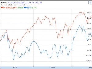
So how similar is your stock to every other one?  How do you know?  Well, for starters your could use Google Finance’s stock comparison tool and take a look at your stock relative to the broader market for the last couple of years:

Note: I used the S&P 500 (via the SPY index fund) as a metric for the broader market.  This is fairly standard.

Now, as you can see, there’s a lot of similarity.  Most of the highs and lows are the same, as is most of the overall movement.  But there are a couple of points of notable divergence – one in 2010 and one in 2011.  In both cases MSFT underperformed the market, and as a result it’s returned 16% less than the market as a whole over this period.  I think Google gets the dividend adjustments right, so this is a legit comparison.

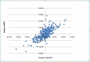
Visually we can say “a lot” of the movement of MSFT stock is driven by the broader market.  But how much, exactly?  Enter the Pearson correlation coefficient, commonly called just the correlation coefficient.  If you’re not comfortable with correlation coefficients, I suggest you at least skim the wikipedia page.  The correlation coefficient can be applied to any two paired groups of numbers – that is, each group of numbers in group 1 has a single counterpart in group 2.  In this case, we’re going to compare the daily price change for MSFT to the daily price change for the S&P500.  For simplicity I’ll go back to the start of 2011.  Visually, the data we’re looking at looks like:

This view makes it even more apparent how closely related the two are.  Now, to calculate the correlation coefficient, we’re going to do all the math on that wiki page.  Just kidding – we’re going to have Excel do it using the CORREL() function.  It works the same in OpenOffice.  Any correlation feature in pretty much any statistics package should be fine too.

Result:  MSFT daily stock price changes are 0.76 correlated to S&P daily price changes

The Pearson correlation coefficient ranges from -1 to 1.  A value of one means the two sets of numbers are perfectly and positively linearly related.  In this case, it would mean that MSFT stock was just a proxy for the S&P.  A value of 0 means there’s no linear relationship to the data.  A value of -1 means they’re perfectly linearly related, but the slope is negative ie MSFT is like owning negative S&P.

So in layman’s terms, we can say they’re 76% the same thing in the positive direction.  Now every clown on the internet will remind you that correlation does not imply causation.  But in this case we can be pretty sure changes in the broader economy cause changes in  MSFT stock price rather than the other way around.  MSFT is big, but they’re not THAT big. So we can say that 76% of changes in MSFT stock price are caused by the broader market.  The remaining 24% are MSFT’s independent movement.

At this point, we’ve successfully chopped the stock into pieces.  One piece behaves like the S&P.  The other piece is MSFT independent of the S&P.  In trader lingo, these pieces are called “alpha” for the independent piece and “beta” for the piece that mirrors the market.  Notice that in the case of MSFT (and most stocks) beta is a much bigger deal than alpha – roughly 3x as much in this case.

We’ve got one more piece of math to do today.  The Pearson correlation coefficient tells you how linearly related two things are.  But it doesn’t tell you the numeric slope of that relationship – just how much it looks like a line.  The slope, however, is very useful.  It allows us to compute the alpha component (we already know what beta looks like – it’s just the S&P).  In order to get the slope, we need to do a least squares linear regression.  Once again, wikipedia has the math, and we’re going to use Excel to save some work.  The function is called LINEST() – just read the documentation I linked, because it’s a little weird.  Not sure how to do it in OpenOffice – this may help.

Result: The slope of the regression line is 0.864

When websites like Google Finance report the “Beta” of a stock, this is what they’re reporting.  There are a couple of different ways to compute beta and different time scales you can use, so reported values won’t be exactly the same.

Now, we can construct MSFT’s alpha component by subtracting out 0.86 * the S&P with everything scaled.  The scaling is a pain in the ass, so if you’re weaksauce on algebra you can just use this formula:

MSFT_ALPHA_CURRENT = MSFT_CURRENT – (MSFT_STARTING * REG_SLOPE * ((S&P_CURRENT – S&P_STARTING)/S&P_STARTING))

Where _STARTING just means the price for that instrument on the first day of your data set.  Never say I didn’t help you 😉

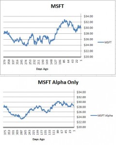
The result:

As you can see, MSFT’s alpha component is a lot less noisy than MSFT itself.  This is consistent with 76% of the movement being caused by the broader market rather than the stock itself.  What’s interesting here is that while most of the short term movement is beta, a lot of the long term movement is alpha.  The alpha component still has multiple 10%+ moves over the last year and a half.

Now, if you’re thinking MSFT’s alpha component looks easier to trade than the stock as a whole, you’re right.  Those big smooth moves are ripe for the picking.  That’s the next place the speculative investing series is going.